Smoothed Aggregation

In order to define the prolongator $P^k$, used to compute the coarse-level matrix $A^{k+1}$, MLD2P4 uses the smoothed aggregation algorithm described in [2,26]. The basic idea of this algorithm is to build a coarse set of indices $\Omega^{k+1}$ by suitably grouping the indices of $\Omega^k$ into disjoint subsets (aggregates), and to define the coarse-to-fine space transfer operator $P^k$ by applying a suitable smoother to a simple piecewise constant prolongation operator, with the aim of improving the quality of the coarse-space correction.

Three main steps can be identified in the smoothed aggregation procedure:

1. aggregation of the indices of $\Omega^k$ to obtain $\Omega^{k+1}$;
2. construction of the prolongator $P^k$;
3. application of $P^k$ and $R^k=(P^k)^T$ to build $A^{k+1}$.

In order to perform the coarsening step, the smoothed aggregation algorithm described in [26] is used. In this algorithm, each index $j \in \Omega^{k+1}$ corresponds to an aggregate $\Omega^k_j$ of $\Omega^k$, consisting of a suitably chosen index $i \in \Omega^k$ and indices that are (usually) contained in a strongly-coupled neighborood of $i$, i.e.,

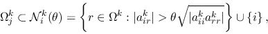$$\Omega^k_j \subset \mathcal{N}_i^k(\theta) = \left\{ r \i... ...vert a_{ii}^ka_{rr}^k\vert} \right \} \cup \left\{ i \right\},$$ (3)

for a given threshold $\theta \in [0,1]$ (see [26] for the details). Since this algorithm has a sequential nature, a decoupled version of it is applied, where each processor independently executes the algorithm on the set of indices assigned to it in the initial data distribution. This version is embarrassingly parallel, since it does not require any data communication. On the other hand, it may produce some nonuniform aggregates and is strongly dependent on the number of processors and on the initial partitioning of the matrix $A$. Nevertheless, this parallel algorithm has been chosen for MLD2P4, since it has been shown to produce good results in practice [5,7,25].

The prolongator $P^k$ is built starting from a tentative prolongator 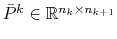$\bar{P}^k \in \mathbb{R}^{n_k \times n_{k+1}}$, defined as

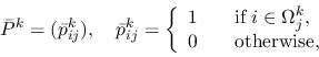$$\bar{P}^k =(\bar{p}_{ij}^k), \quad \bar{p}_{ij}^k = \left\{... ...Omega^k_j, \\ 0 & \quad \mbox{otherwise}, \end{array} \right.$$ (4)

where $\Omega^k_j$ is the aggregate of $\Omega^k$ corresponding to the index $j \in \Omega^{k+1}$. $P^k$ is obtained by applying to $\bar{P}^k$ a smoother $S^k \in \mathbb{R}^{n_k \times n_k}$:

$$P^k = S^k \bar{P}^k,$$

in order to remove nonsmooth components from the range of the prolongator, and hence to improve the convergence properties of the multilevel method [2,24]. A simple choice for $S^k$ is the damped Jacobi smoother:

$$S^k = I - \omega^k (D^k)^{-1} A^k_F ,$$

where $D^k$ is the diagonal matrix with the same diagonal entries as $A^k$, $A^k_F = (\bar{a}_{ij}^k)$ is the filtered matrix defined as

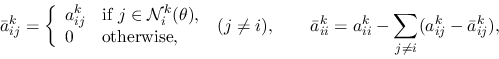$$\bar{a}_{ij}^k = \left \{ \begin{array}{ll} a_{ij}^k & \m... ...ii}^k = a_{ii}^k - \sum_{j \ne i} (a_{ij}^k - \bar{a}_{ij}^k),$$ (5)

and $\omega^k$ is an approximation of $4/(3\rho^k)$, where $\rho^k$ is the spectral radius of $(D^k)^{-1}A^k_F$ [2]. In MLD2P4 this approximation is obtained by using $\Vert A^k_F \Vert _\infty$ as an estimate of $\rho^k$. Note that for systems coming from uniformly elliptic problems, filtering the matrix $A^k$ has little or no effect, and $A^k$ can be used instead of $A^k_F$. The latter choice is the default in MLD2P4.