Multi-level Schwarz Preconditioners

The Multilevel preconditioners implemented in MLD2P4 are obtained by combining AS preconditioners with coarse-space corrections; therefore we first provide a sketch of the AS preconditioners.

Given the linear system , where $A=(a_{ij}) \in \Re^{n \times n}$ is a nonsingular sparse matrix with a symmetric nonzero pattern, let $G=(W,E)$ be the adjacency graph of $A$, where $W=\{1, 2, \ldots, n\}$ and $E=\{(i,j) : a_{ij} \neq 0\}$ are the vertex set and the edge set of $G$, respectively. Two vertices are called adjacent if there is an edge connecting them. For any integer $\delta > 0$, a $\delta$-overlap partition of $W$ can be defined recursively as follows. Given a 0-overlap (or non-overlapping) partition of $W$, i.e. a set of $m$ disjoint nonempty sets $W_i^0 \subset W$ such that $\cup_{i=1}^m W_i^0 = W$, a $\delta$-overlap partition of $W$ is obtained by considering the sets $W_i^\delta \supset W_i^{\delta-1}$ obtained by including the vertices that are adjacent to any vertex in $W_i^{\delta-1}$.

Let $n_i^\delta$ be the size of $W_i^\delta$ and $R_i^{\delta} \in \Re^{n_i^\delta \times n}$ the restriction operator that maps a vector $v \in \Re^n$ onto the vector $v_i^{\delta} \in \Re^{n_i^\delta}$ containing the components of $v$ corresponding to the vertices in $W_i^\delta$. The transpose of $R_i^{\delta}$ is a prolongation operator from $\Re^{n_i^\delta}$ to $\Re^n$. The matrix $A_i^\delta=R_i^\delta A (R_i^\delta)^T \in \Re^{n_i^\delta \times n_i^\delta}$ can be considered as a restriction of $A$ corresponding to the set $W_i^{\delta}$.

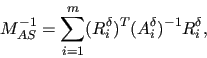
The classical one-level AS preconditioner is defined by

$$M_{AS}^{-1}= \sum_{i=1}^m (R_i^{\delta})^T (A_i^\delta)^{-1} R_i^{\delta},$$

where $A_i^\delta$ is assumed to be nonsingular. Its application to a vector $v \in \Re^n$ within a Krylov solver requires the following three steps:

1. restriction of $v$ as $v_i = R_i^{\delta} v$, $i=1,\ldots,m$;
2. solution of the linear systems $A_i^\delta w_i = v_i$, $i=1,\ldots,m$;
3. prolongation and sum of the $w_i$'s, i.e. $w = \sum_{i=1}^m (R_i^{\delta})^T w_i$.

Note that the linear systems at step 2 are usually solved approximately, e.g. using incomplete LU factorizations such as ILU($p$), MILU($p$) and ILU($p,t$) [22, Chapter 10].

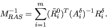
A variant of the classical AS preconditioner that outperforms it in terms of convergence rate and of computation and communication time on parallel distributed-memory computers is the so-called Restricted AS (RAS) preconditioner [5,15]. It is obtained by zeroing the components of $w_i$ corresponding to the overlapping vertices when applying the prolongation. Therefore, RAS differs from classical AS by the prolongation operators, which are substituted by $(\tilde{R}_i^0)^T \in \Re^{n_i^\delta \times n}$, where $\tilde{R}_i^0$ is obtained by zeroing the rows of $R_i^\delta$ corresponding to the vertices in $W_i^\delta \backslash W_i^0$:

$$M_{RAS}^{-1}= \sum_{i=1}^m (\tilde{R}_i^0)^T (A_i^\delta)^{-1} R_i^{\delta}.$$

Analogously, the AS variant called AS with Harmonic extension (ASH) is defined by

$$M_{ASH}^{-1}= \sum_{i=1}^m (R_i^{\delta})^T (A_i^\delta)^{-1} \tilde{R}_i^0.$$

We note that for $\delta=0$ the three variants of the AS preconditioner are all equal to the block-Jacobi preconditioner.

As already observed, the convergence rate of the one-level Schwarz preconditioned iterative solvers deteriorates as the number $m$ of partitions of $W$ increases [7,23]. To reduce the dependency of the number of iterations on the degree of parallelism we may introduce a global coupling among the overlapping partitions by defining a coarse-space approximation $A_C$ of the matrix $A$. In a pure algebraic setting, $A_C$ is usually built with the Galerkin approach. Given a set $W_C$ of coarse vertices, with size $n_C$, and a suitable restriction operator $R_C \in \Re^{n_C \times n}$, $A_C$ is defined as

$$A_C=R_C A R_C^T$$

and the coarse-level correction matrix to be combined with a generic one-level AS preconditioner $M_{1L}$ is obtained as

$$M_{C}^{-1}= R_C^T A_C^{-1} R_C,$$

where $A_C$ is assumed to be nonsingular. The application of $M_{C}^{-1}$ to a vector $v$ corresponds to a restriction, a solution and a prolongation step; the solution step, involving the matrix $A_C$, may be carried out also approximately.

The combination of $M_{C}$ and $M_{1L}$ may be performed in either an additive or a multiplicative framework. In the former case, the two-level additive Schwarz preconditioner is obtained:

$$M_{2LA}^{-1} = M_{C}^{-1} + M_{1L}^{-1}.$$

Applying $M_{2L-A}^{-1}$ to a vector $v$ within a Krylov solver corresponds to applying $M_{C}^{-1}$ and $M_{1L}^{-1}$ to $v$ independently and then summing up the results.

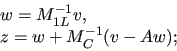
In the multiplicative case, the combination can be performed by first applying the smoother $M_{1L}^{-1}$ and then the coarse-level correction operator $M_{C}^{-1}$:

$$\begin{array}{l} w = M_{1L}^{-1} v, \\ z = w + M_{C}^{-1} (v-Aw); \end{array}$$

this corresponds to the following two-level hybrid pre-smoothed Schwarz preconditioner:

$$M_{2LH-PRE}^{-1} = M_{C}^{-1} + \left( I - M_{C}^{-1}A \right) M_{1L}^{-1}.$$

On the other hand, by applying the smoother after the coarse-level correction, i.e. by computing

$$\begin{array}{l} w = M_{C}^{-1} v , \\ z = w + M_{1L}^{-1} (v-Aw) , \end{array}$$

the two-level hybrid post-smoothed Schwarz preconditioner is obtained:

$$M_{2LH-POST}^{-1} = M_{1L}^{-1} + \left( I - M_{1L}^{-1}A \right) M_{C}^{-1}.$$

One more variant of two-level hybrid preconditioner is obtained by applying the smoother before and after the coarse-level correction. In this case, the preconditioner is symmetric if $A$, $M_{1L}$ and $M_{C}$ are symmetric.

As previously noted, on parallel computers the number of submatrices usually matches the number of available processors. When the size of the system to be preconditioned is very large, the use of many processors, i.e. of many small submatrices, often leads to a large coarse-level system, whose solution may be computationally expensive. On the other hand, the use of few processors often leads to local sumatrices that are too expensive to be processed on single processors, because of memory and/or computing requirements. Therefore, it seems natural to use a recursive approach, in which the coarse-level correction is re-applied starting from the current coarse-level system. The corresponding preconditioners, called multi-level preconditioners, can significantly reduce the computational cost of preconditioning with respect to the two-level case (see [23, Chapter 3]). Additive and hybrid multilevel preconditioners are obtained as direct extensions of the two-level counterparts. For a detailed descrition of them, the reader is referred to [23, Chapter 3]. The algorithm for the application of a multi-level hybrid post-smoothed preconditioner $M$ to a vector $v$, i.e. for the computation of $w=M^{-1}v$, is reported, for example, in Figure 1. Here the number of levels is denoted by $nlev$ and the levels are numbered in increasing order starting from the finest one, i.e. the finest level is level 1; the coarse matrix and the corresponding basic preconditioner at each level $l$ are denoted by $A_l$ and $M_l$, respectively, with $A_1=A$, while the related restriction operator is denoted by $R_l$.

Figure 1: Application of the multi-level hybrid post-smoothed preconditioner.